Columnar Storage Explained: How Columns, Sort Order and Codecs Shrink Your Data

Two copies of the same data can differ in size by more than six times. Same rows, same values, nothing deleted. The only difference is how the bytes are laid out on disk: row by row or column by column, in arrival order or sorted, and which encoding and compression codec squeezes them.

In the first Byte2MB edition we turned events into gigabytes. In the second we saw how retention multiplies them. This edition is about the bytes you decide to keep: how columnar storage, sort order and compression codecs make them smaller and faster to query. To keep it honest, we ran an experiment on one million synthetic log rows and measured every number below.

Rows vs columns

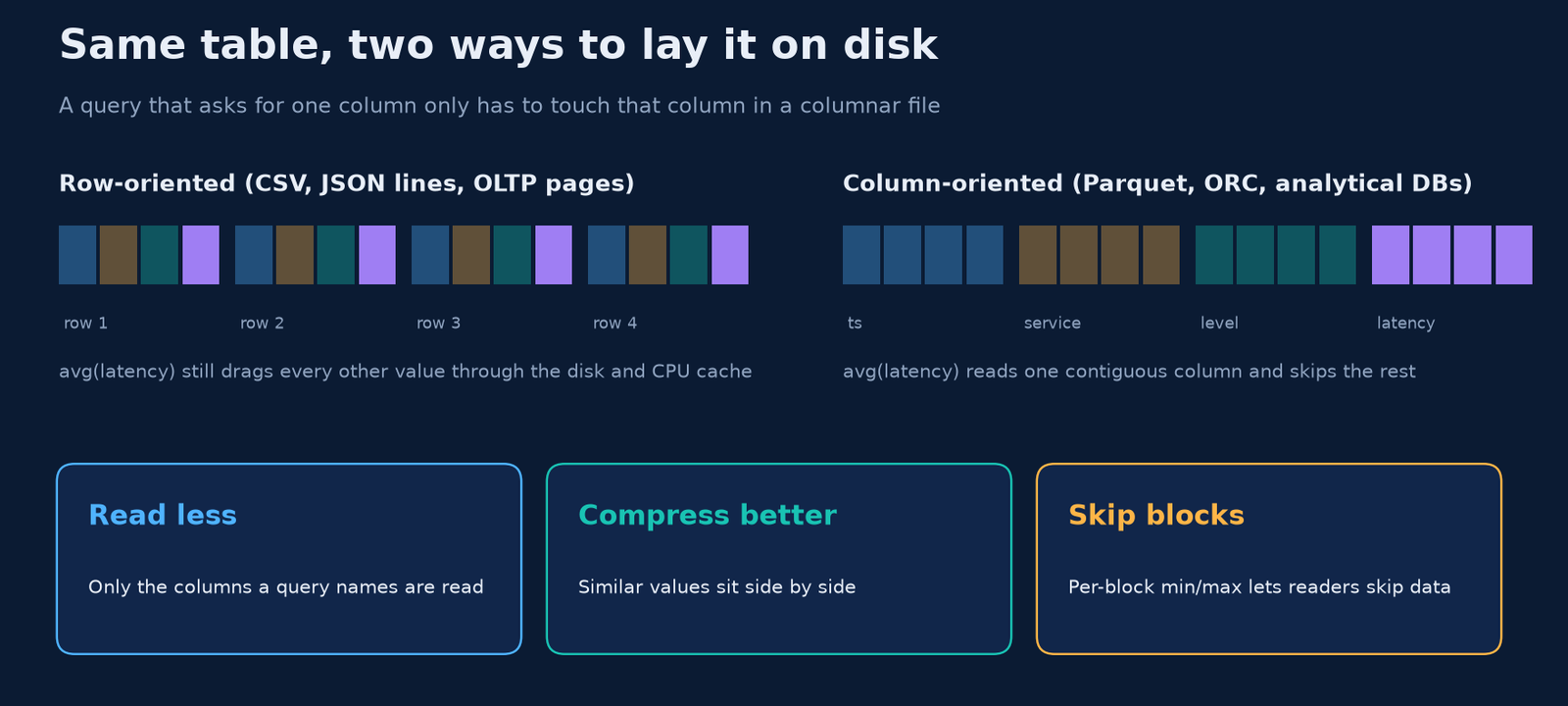
A CSV file, a JSON-lines log or a classic transactional database page stores data row by row: every field of row 1, then every field of row 2, and so on. That’s ideal when you read or write whole records, one at a time.

Analytical queries look different. avg(latency) over a day of logs needs one field from millions of rows. In a row layout, the reader still has to pull every other field through disk and memory to get there.

A columnar format such as Parquet, or a column-oriented database, stores each column’s values together. The Parquet file format splits a table into row groups, and inside each row group keeps one column chunk per column. A footer at the end records where every chunk starts, so a reader can fetch only the columns a query names.

Our experiment: one million log rows

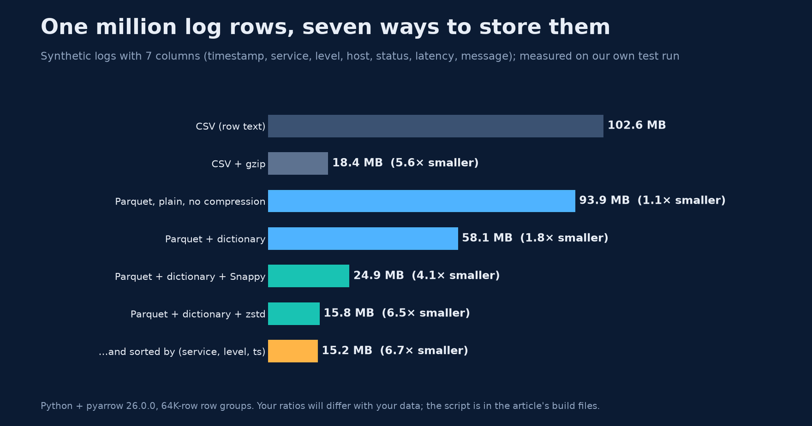
We generated one million synthetic log rows covering one day, with seven columns: timestamp, service (20 values), level (DEBUG, INFO, WARN, ERROR), host (200 values), HTTP status, latency, and a free-text message containing a path, an order ID and the latency. Then we wrote the exact same rows in seven ways using Python and pyarrow, and measured the file sizes.

A few things stand out:

• Columnar alone is not magic. Plain, uncompressed Parquet was 93.9 MB, barely smaller than the 102.6 MB CSV. The layout sets the stage. Encodings and codecs do the work.
• Encoding came first. Turning on dictionary encoding cut the file to 58.1 MB with no general-purpose compression at all.
• The codec matters. Snappy brought it to 24.9 MB and zstd to 15.8 MB, about 6.5× smaller than the CSV. That’s roughly 103 bytes per row down to about 16.
• Gzip on CSV gets close on size (18.4 MB), but you lose everything else: you must decompress and parse every column to answer any question.

Encodings: shrink before you compress

Columnar formats apply cheap, type-aware encodings before a general-purpose codec ever runs. The Parquet encoding spec defines several, and two do most of the heavy lifting for logs and metrics:

• Dictionary encoding stores each distinct value once, then replaces the values with small integer IDs that are run-length and bit-packed. A column like level with four distinct values becomes a stream of 2-bit numbers. If the dictionary grows too big, the writer falls back to plain encoding.
• Delta encoding (DELTA_BINARY_PACKED) stores the differences between consecutive integers instead of the integers themselves. Timestamps that tick forward a few milliseconds at a time turn into tiny numbers.

We tested the timestamp column on its own. As raw 64-bit integers it’s 8.0 MB. Plain encoding plus zstd gave 1.56 MB. Delta encoding alone gave 1.17 MB, and delta plus zstd 1.11 MB. (In the full-table files we kept pyarrow’s default settings, which also tried dictionary encoding on the timestamps, so that column shows up larger in the next chart.) Databases offer the same idea as column codecs: ClickHouse, for example, lets you write CODEC(Delta, ZSTD) on a column, and its CREATE TABLE docs note that it uses LZ4 by default when self-managed and zstd in its cloud service.

Want to see what this means for your own tables? Plug in your row count, row size and how many columns a typical query touches:

Sort order: put similar values side by side

Compression works by finding repetition. If rows arrive in time order, the service column looks like a random shuffle of 20 names. Sort the rows by service first, and the same column becomes 20 long runs of identical values.

We re-wrote the million rows sorted by (service, level, timestamp) and compared each column’s compressed size:

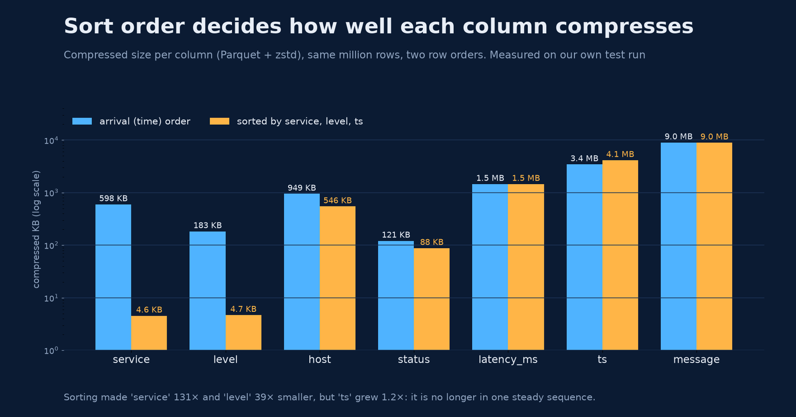
The service column went from 598 KB to 4.6 KB, about 131× smaller, and level about 39× smaller. host, which follows service, nearly halved. But the timestamp column grew from 3.4 MB to 4.1 MB, because it’s no longer one steady sequence. Overall the file went from 15.8 MB to 15.2 MB. The free-text message column, at 9.0 MB, didn’t care either way. High-entropy text is often your biggest column, and sorting can’t fix it.

Order also matters the other way round. When we shuffled the rows randomly, the zstd file grew to 18.2 MB, about 15% bigger than arrival order.

ClickHouse’s guide to primary indexes shows the same effect at larger scale. On 8.87 million rows of web traffic, ordering the key columns from low to high cardinality, (IsRobot, UserID, URL), left the UserID column at 877.47 KiB, versus 11.24 MiB with the opposite order: a compression ratio of 39 instead of 3. The rule of thumb is to put low-cardinality columns you filter on first.

Skipping: the fastest byte is the one you don’t read

Columnar files keep lightweight statistics for each block, such as the minimum and maximum value of every column in every row group. A reader checks those first and skips any block whose range can’t contain a match.

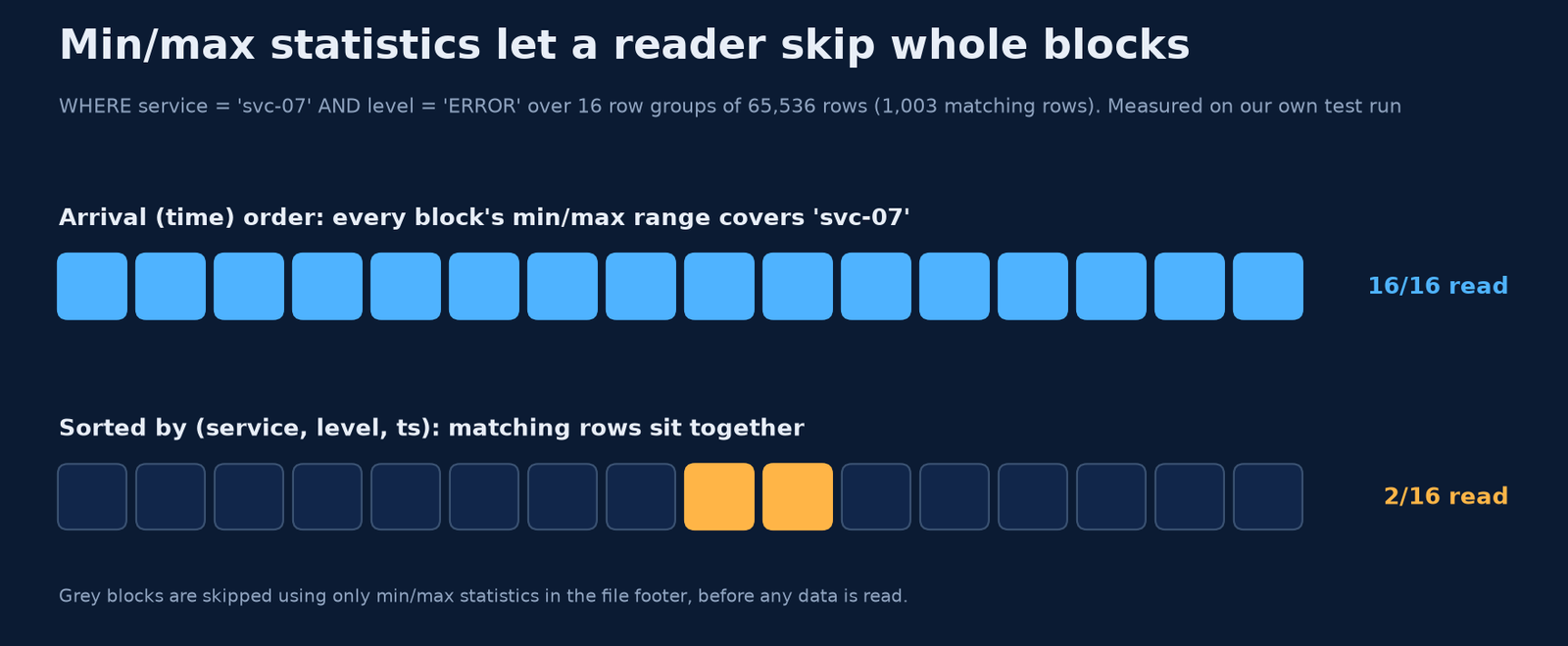
For WHERE service = 'svc-07' AND level = 'ERROR' (1,003 matching rows), every one of our 16 row groups had a min/max range covering svc-07 in arrival order, so none could be skipped. In the sorted file, only 2 of 16 needed reading. Combine that with column pruning: that query needs three of seven columns, which were just 14% of the compressed file.

Databases do the same at finer grain. ClickHouse’s sparse primary index stores one entry per granule, 8,192 rows by default, and in its guide a lookup on the first key column selected 1 of 1,083 granules instead of scanning all 8.87 million rows.

A practical checklist

1. Store analytical data in a columnar format, not CSV or JSON lines.
2. Make sure encodings are on. Dictionary for repetitive strings, delta for timestamps and counters.
3. Pick a codec on purpose. zstd gave the smallest file in our test; lighter codecs such as LZ4 and Snappy are usually chosen for speed. Measure size and speed on your own data.
4. Sort by what you filter on, low-cardinality columns first, then time.
5. Keep blocks a sensible size so min/max statistics can actually skip data.
6. Select only the columns you need. SELECT * throws away the columnar advantage.
7. Watch your fattest column. Free-text messages often dominate; consider extracting structured fields.

Sources: Apache Parquet, File format · Apache Parquet, Encodings · ClickHouse, CREATE TABLE: column compression codecs · ClickHouse, A practical introduction to primary indexes. All file sizes, column sizes and row-group counts come from Byte2MB’s own test on one million synthetic log rows (Python, pyarrow 26.0.0); the script is available on request.