Predicate Pushdown and Partition Pruning: How Queries Skip 99% of Your Data

The fastest data is the data you never read. When an analytics query returns in milliseconds over billions of rows, the database usually hasn’t scanned quickly. It has worked out which files, blocks and columns can’t contain the answer, and skipped them.

That skipping goes by a few names: predicate pushdown, partition pruning, data skipping. Earlier Byte2MB editions sized, retained and compressed data. This one is about reading it, with every byte below measured in our own reproducible test on synthetic data.

What predicate pushdown means

A predicate is the filter in your query: WHERE service = 'checkout' AND ts >= '2026-01-15'. Pushing it down means handing that filter to the storage layer, so the reader can rule data out before it’s loaded and decoded, instead of reading everything and filtering afterwards.

It only works because storage keeps small summaries next to the data. Columnar formats like Parquet store min/max statistics at several levels, such as per column chunk and per page, according to the Parquet format specification. If a block’s timestamps run from 3 January to 4 January, a query for 15 January can skip it without opening it.

Four ways a query avoids reading data

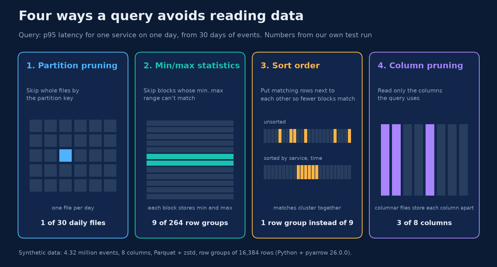
1. Partition pruning. Data is split into separate files or parts by a partition key, often the day. A query for one day ignores the other 29 files entirely.
2. Min/max statistics. Inside each file, data sits in blocks (row groups in Parquet, granules in ClickHouse). If a block’s min..max range can’t match the filter, it’s skipped.
3. Sort order. Statistics only help when matching rows are close together. Sorting by the columns you filter on puts them in a handful of blocks instead of spreading them across all of them.
4. Column pruning. Columnar storage keeps each column apart, so a query that needs 3 columns doesn’t pay for the other 5.

Our experiment: one query, five layouts

We generated 4.32 million synthetic API events over 30 days, with 8 columns: timestamp, service (50 values), endpoint, status, latency, response bytes, request ID and user ID. We wrote them as Parquet (zstd, row groups of 16,384 rows) in five layouts, using Python and pyarrow with a fixed seed. It’s a storage model, not a specific database: the ratios are the lesson.

The query: p95 latency for one service on one day. That’s 2,936 matching rows out of 4,320,000. For each layout we added up the compressed bytes a reader must fetch after pruning, straight from the Parquet metadata, and ran the real filtered read to check it returned the same rows.

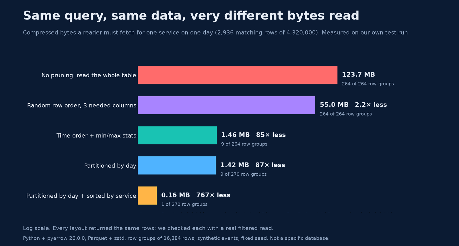
• Reading everything meant 123.7 MB across all 264 row groups.
• Column pruning alone, on data in random row order, cut that to 55.0 MB. But the min/max statistics skipped nothing: when rows are shuffled, every block holds every service and every day.
• Time order, which is how most event data arrives, let the statistics skip 255 of 264 row groups: 1.46 MB read.
• Partitioning by day read 1.42 MB, about the same, because the data was already in time order. It did mean opening only 1 of 30 files.
• Sorting each day by service, then time put all of one service’s rows in a single row group: 0.16 MB, 767 times less than the full scan.

The layout of the data, not the query, decided whether 99.9% of the bytes could be skipped.

Partitioning is not the same as indexing

Our partitioned and unpartitioned time-ordered files read almost the same bytes. That matches the ClickHouse partitions guide: partitioning is primarily a data management feature, for dropping or moving old data, and helps queries mainly when the partition key isn’t already in the sort key. It also warns that querying across all partitions is typically slower than on a non-partitioned table, and recommends a partition key with cardinality under 1,000 to 10,000.

In short: partition by something coarse, like day or month, that matches how you delete data. Sort by what you filter on.

Sparse indexes: one entry per block, not per row

Analytical databases often skip data with a sparse primary index. Instead of one index entry per row, as in a B-tree, it stores the key of the first row of every block of rows. The ClickHouse primary index guide describes one entry (“mark”) per granule of 8,192 rows by default, giving 1,083 marks for its 8.87-million-row example. Small enough to fit in memory, which it must. In that guide, a query that did a full scan of 8.87 million rows read only 8.19 thousand rows once the table had a fitting primary key.

We simulated the same idea on our data, sorted by (service, time), and changed the block size.

Small granules made the index big (16,875 entries at 256 rows) but read little extra: 3,328 rows for 2,936 matches. Huge granules made it tiny (33 entries) but read 131,072 rows. At 8,192 rows per granule, 528 entries and 16,384 rows read, about 5.6 times the matches: a modest price for an index that fits in RAM.

Block size cuts both ways in file formats too. The Parquet configuration docs recommend large row groups (512 MB to 1 GB) for big sequential reads. Large row groups mean better scan throughput but coarser skipping.

Try it: data skipping estimator

Plug in your own table and query, and see what each technique saves.

How to make your queries skip more

1. Sort by what you filter on. Put the columns most queries filter on first in the sort or primary key. ClickHouse’s guide also suggests ordering key columns from low to high cardinality.
2. Keep time in the layout. Most observability queries ask for a time window, so put time in the partition key, the sort key, or both.
3. Partition coarsely. Day or month, aligned with retention. Thousands of tiny partitions create the small-files problem and slow every query that spans them.
4. Select only what you need. SELECT * turns off column pruning.
5. Write filters the storage can use. Compare the raw column to a constant. Wrapping a column in a function can stop the engine from using the stored statistics.
6. Check the plan. Most engines can show how many partitions and blocks a query will read (for example EXPLAIN indexes = 1 in ClickHouse). If it says “all of them”, the layout is working against you.

Sources: Apache Parquet, Format specification · Apache Parquet, Configurations · ClickHouse, A practical introduction to primary indexes · ClickHouse, Table partitions. All bytes read, row groups, index entries and rows read come from Byte2MB’s own test on synthetic events (4.32 million rows, Python, pyarrow 26.0.0, Parquet + zstd, fixed seed). The script is available on request.