Hot, Warm, Cold: How Data Retention Multiplies Your Observability Storage

Most observability data is read once, if ever. You look at the last hour of logs during an incident, the last day of metrics on a dashboard, and maybe last month’s trend when someone asks for a report. Yet many systems keep every byte at full resolution, on the same fast disks, for as long as anyone can remember.

In the first Byte2MB edition we saw how a modest 1 KB event at 1,000 events per second becomes 86.4 GB a day. This edition is about the other half of that equation: how long you keep it, where you keep it, and in how much detail. That’s retention and tiering, and it’s often the biggest lever you have on storage size.

Retention is a multiplier

The amount of data you hold at any moment is simple to write down:

stored data = daily volume × retention days × copies

Ingest rate gets all the attention, but retention multiplies it quietly. Take that same 86.4 GB/day stream and keep a single copy:

• 7 days: 86.4 × 7 = 604.8 GB
• 30 days: 86.4 × 30 = 2,592 GB (about 2.6 TB)
• 90 days: 86.4 × 90 = 7,776 GB (about 7.8 TB)
• 365 days: 86.4 × 365 = 31,536 GB (about 31.5 TB)

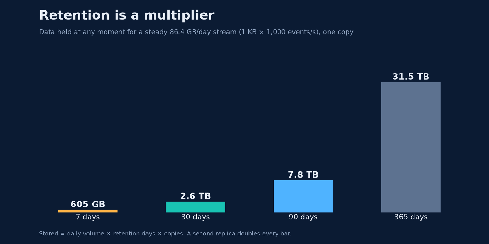
Add a replica for durability and every number doubles. Nothing about the workload changed. Only the policy did.

Want to try this with your own numbers? Plug your event size, rate and retention into the estimator below:

Not all data needs the same home

The fix is not “keep less” across the board. It’s to notice that the value of observability data drops as it ages, while the cost of storing it stays the same unless you move it. That’s the idea behind tiering: put recent data on fast, expensive storage and older data on slower, cheaper storage, then delete it when nobody needs it.

Elasticsearch’s index lifecycle management names the phases clearly: hot (actively written and queried), warm (no longer written, still queried), cold (queried rarely, slower is fine), frozen (queried very rarely, very slow is fine) and delete. Other systems use different words, but the shape is the same.

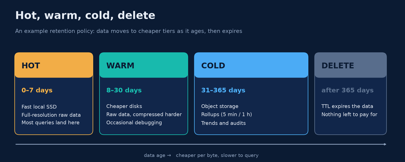
Look at what tiering does to the 90-day example. If only the last 7 days are hot, the hot tier holds 604.8 GB, which is 7 ÷ 90, or about 7.8%, of the 7,776 GB total. The other 7,171.2 GB still exist, but on storage that costs less per byte. You haven’t thrown anything away. You’ve just stopped paying premium rates for data nobody is querying.

TTLs: let the database do the moving

You don’t need a cron job for this. Most time-series and analytical databases let you declare the policy on the table and enforce it automatically.

In ClickHouse, a TTL clause can delete rows, move data to another disk or volume, or roll rows up into aggregates once they pass a certain age. A hot/warm/cold setup is a few lines, for example TTL ts TO VOLUME 'hot', ts + INTERVAL 7 DAY TO VOLUME 'warm', ts + INTERVAL 30 DAY TO VOLUME 'cold'. Two practical details from the ClickHouse TTL guide are worth knowing:

• TTL rules are applied during background merges, not the instant data expires. By default delete TTLs are re-checked at least every 4 hours (merge_with_ttl_timeout = 14,400 seconds).
• Partition by the same time column you use in the TTL. Then ClickHouse can drop whole partitions instead of rewriting parts row by row.

Prometheus has a simpler model: one retention window, --storage.tsdb.retention.time, which defaults to 15 days if you set neither a time nor a size limit (Prometheus storage docs). Long-term systems layered on top usually add tiers and downsampling.

Downsampling: keep the shape, drop the detail

For metrics, there is a second lever beyond moving data: downsampling, also called rollups. Instead of keeping a sample every 10 seconds forever, you keep one summary per 5 minutes or per hour.

The arithmetic is striking. A series scraped every 10 seconds produces 86,400 ÷ 10 = 8,640 samples a day. At 5-minute resolution that’s 288 points a day, and at 1-hour resolution, 24.

To check how that translates into bytes, we generated 50 synthetic gauge series (think CPU usage, with a daily cycle, noise and rare spikes) at 10-second resolution for 30 days. That’s 12,960,000 samples. We stored them as Parquet with zstd compression, then built 5-minute and 1-hour rollups that keep four values per bucket: min, max, sum and count.

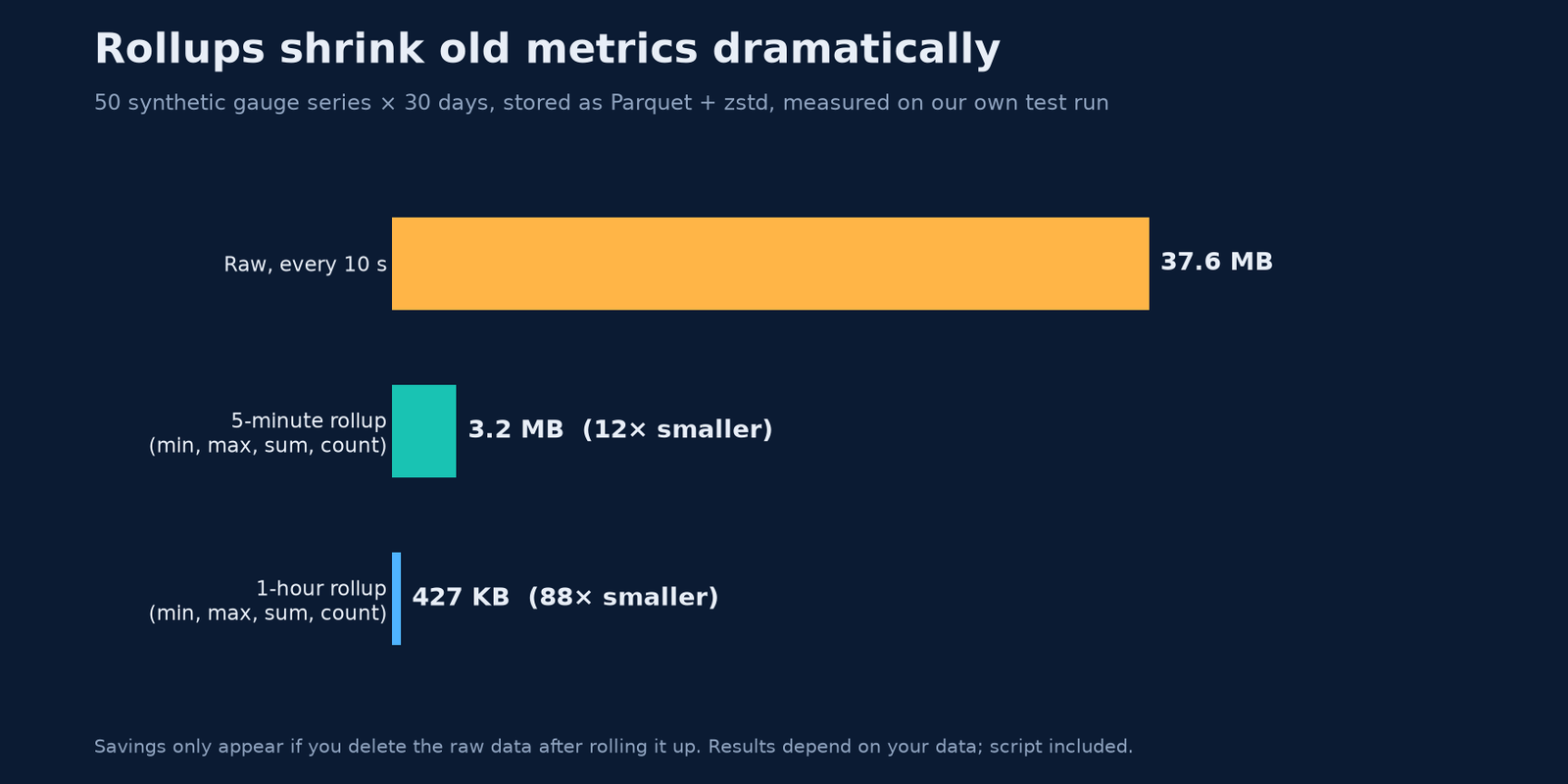
On this sample, the 5-minute rollup was about 12× smaller and the 1-hour rollup about 88× smaller than the raw data. Synthetic data is tidier than real metrics, so treat these as a direction, not a promise.

One important catch: rollups only save space if you delete the raw data afterwards. The Thanos compactor docs are refreshingly honest here. Thanos creates 5-minute downsampled blocks for data older than 40 hours and 1-hour blocks for data older than 10 days, mainly to make long-range queries fast. If you keep all three resolutions, it warns that total storage can grow by up to about 3×. The savings come from giving each resolution its own, shorter retention.

Why rollups keep min and max

An average is a lossy summary. A one-minute CPU spike inside a 5-minute window almost disappears when you average it with four quiet minutes.

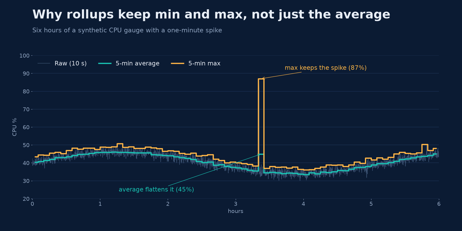
That’s why good rollups store several aggregates. Elasticsearch’s downsample action keeps min, max, sum, value_count and avg for each metric field. Thanos keeps count, sum, min, max and a counter. With sum and count you can still compute a correct average over any longer window. With max, the spike survives.

A practical retention checklist

1. Write down how people query. How far back do incident investigations go? Dashboards? Audits? Let that set your tier boundaries.
2. Do the multiplication. Daily volume × retention × copies, per tier, before you buy disks.
3. Separate logs from metrics. Logs rarely roll up well. Metrics roll up beautifully.
4. Roll up, then expire the raw data. Keeping every resolution forever defeats the purpose.
5. Keep min, max, sum and count in rollups, not just the average.
6. Let TTLs enforce it, and align partitions with the TTL column.
7. Treat deletion as a feature. Data you don’t keep is data you never pay for, back up or secure.

Sources: ClickHouse, Manage data with TTL · Prometheus, Storage · Thanos, Compactor and downsampling · Elastic, Index lifecycle management phases and actions. The rollup and spike figures come from Byte2MB’s own test on synthetic data; the script is available on request.